
How to Compare Columns in Google Sheets: Use Cases

Learn how to compare two columns in Google Sheets to find duplicates, highlight differences, remove duplicate values, or match case-sensitive data without complex formulas, using real-life use cases.
How to compare two columns in Google Sheets
To compare two columns without complex formulas, use Compare Columns (opens in a new tab) (available as part of Compare Sheets (opens in a new tab) or Power Tools (opens in a new tab)):
- Launch the tool depending on your installed add-on:
- Via Power Tools: Go to .
- Via Compare Sheets: Go to .
- Select your Main Column and Compared Column.
- Pick your comparison mode: Duplicate (matches) or Unique (differences).
- Choose an action: Fill with color, Add a status column, Copy / Move to another location, Delete cells / Clear values.
- Click Compare.
Why the add-on is better than standard formulas:
| Feature | Standard Formulas | Compare Columns |
|---|---|---|
| Setup speed | Slow: manual formula creation | Instant: Set up comparison mode and click “Compare” |
| Case sensitivity | Complex: EXACT + ARRAYFORMULA | Single checkbox: Match case |
| Handling blank cells | Requires nested IF logic | Built-in: Skip empty cells |
| Actions available | Limited: • Text results in helper columns • Color fill via custom conditional formatting formulas • Deleting or moving rows must be done manually | Automated actions: • Fill with color • Add a status column • Copy/Move to another location • Delete entire rows from the sheet • Delete cells and shift data up • Clear values |
Let’s see how it works in real-world scenarios 👉.
Case 1: Reconciling Invoices: compare two columns and highlight unpaid bills
Scenario:
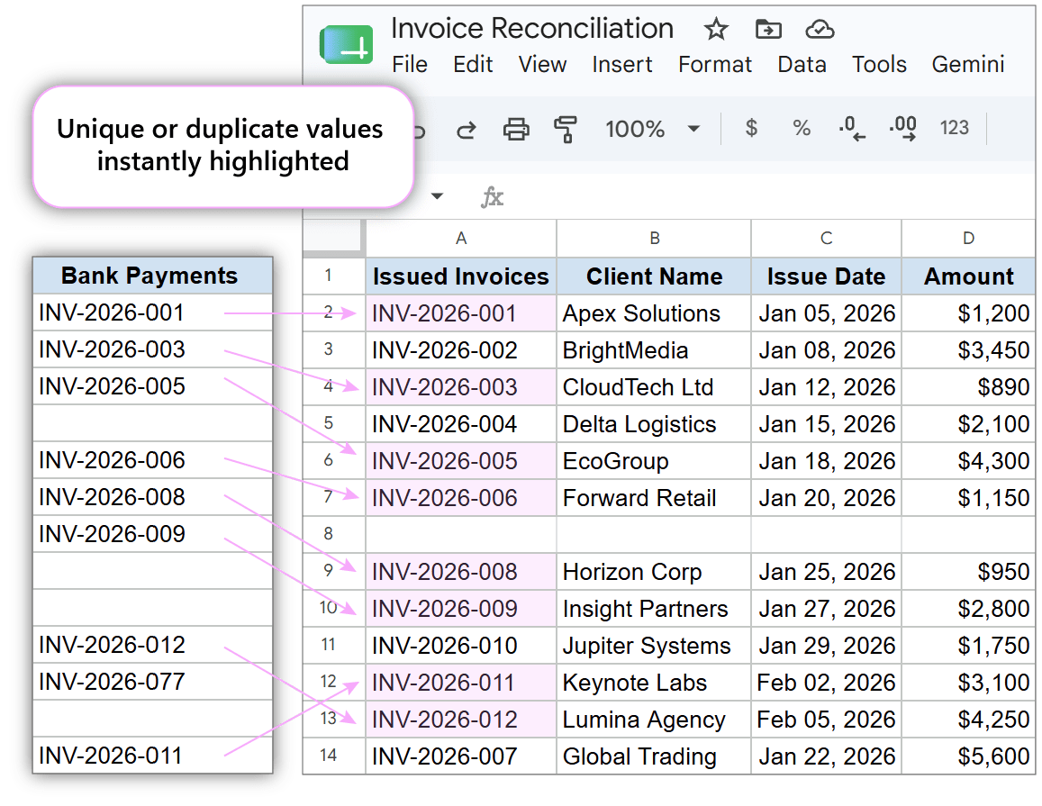
A finance manager has a list of all issued invoices in one column and a list of paid invoices in another one. The goal is to quickly identify all unpaid invoices.
Problem:
- Extra columns: If you use formulas like
=COUNTIF()(opens in a new tab) or=MATCH()(opens in a new tab), you have to create a separate helper column and drag formulas down thousands of rows to highlight missing entries. - Blank cells: Standard formulas often process blank cells as zero or actual data, leading to false matches.
- Custom formula lags: You can color-code unpaid invoices with conditional formatting, but to set it up you’ll need a custom formula like
=ISNA(MATCH(...)), which can lag heavily on large files.
Learn about conditional formatting in Google Sheets (opens in a new tab) in our dedicated guide.
Solution:
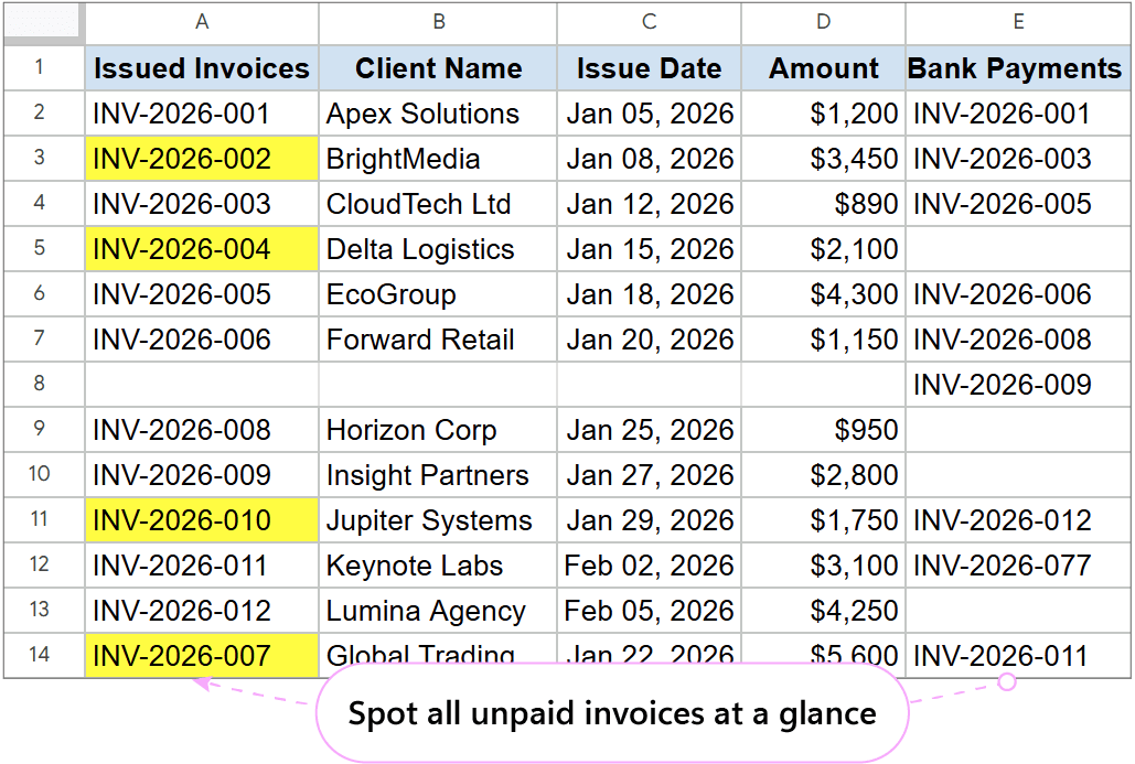
The Compare Columns tool compares columns highlighting unpaid invoices directly inside your original list.
How it works:
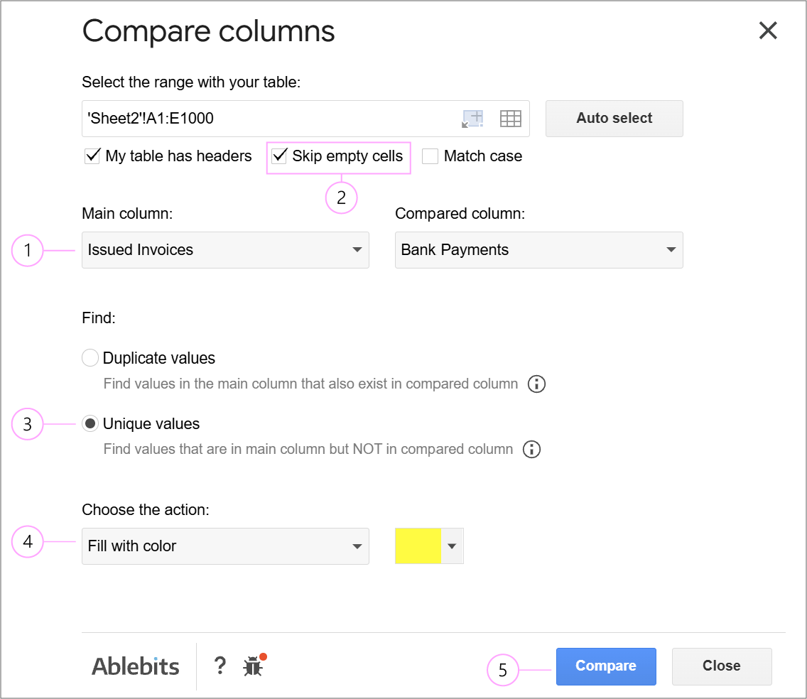
- Select your columns: Launch the add-on and select a column with issued invoices as your main column, and the column with received payments as your compared column.
- Adjust additional settings: Check the Skip empty cells box so the tool ignores blank rows in your bank statement export and avoids false matches.
- Choose comparison mode: Select Unique values to find invoices that exist in the issued list but are missing from the paid list.
- Select an action: Choose Fill with color to highlight unpaid invoices directly in the list.
- Run the tool: Click Compare.
Key Benefit:
- No helper columns: Identifies and acts on unique values directly within your existing sheet structure.
- Handles blank cells: Settings like Skip empty cells ensure blank rows don’t trigger false matches.
- Quick results: Automates reconciliation, eliminates manual scanning, and reduces the risk of missing overdue payments.
Case 2: Cleaning up email lists by removing unsubscribed contacts (delete matches)
Scenario:
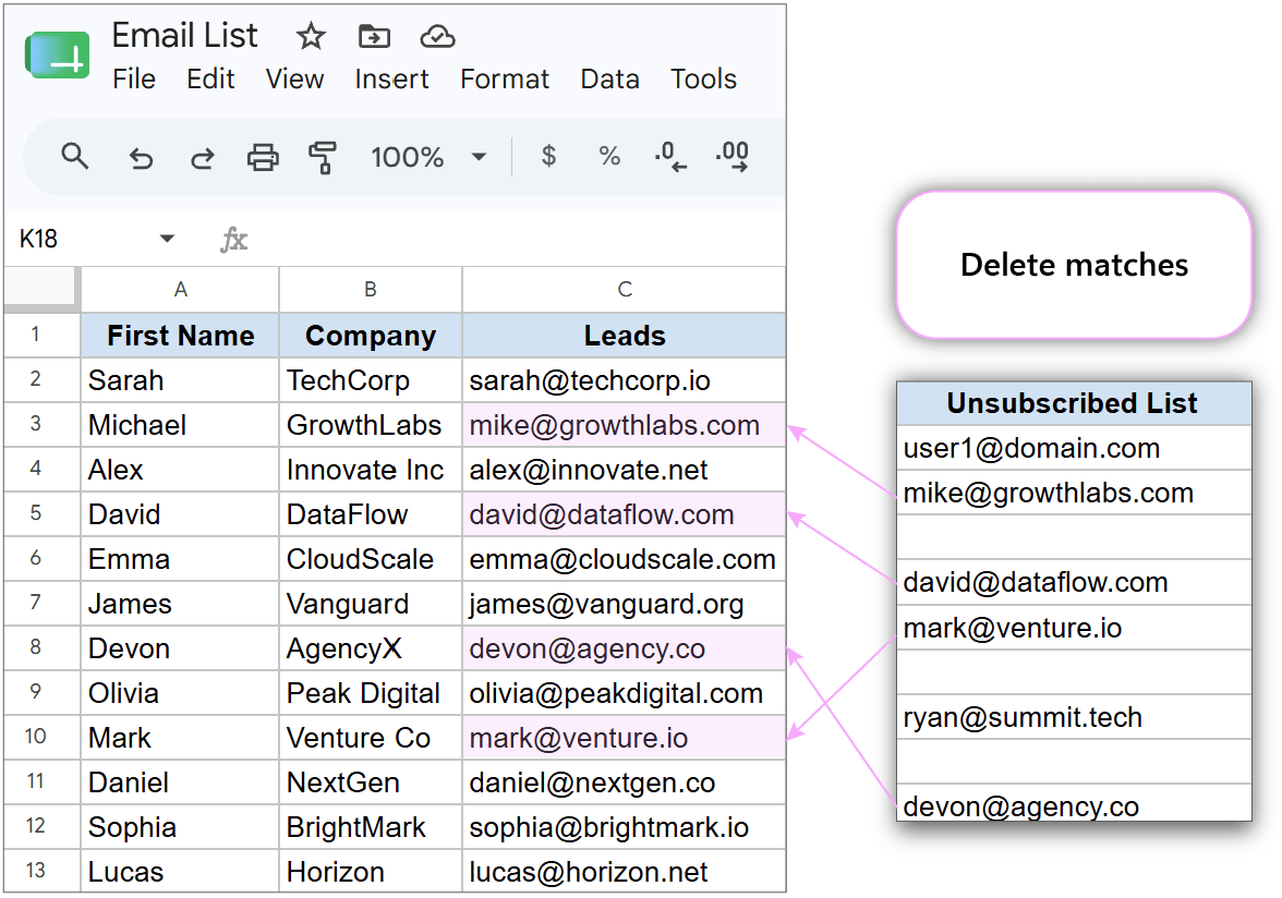
A marketing manager is preparing a newsletter campaign. There is a primary email list of target leads in one column and a list of unsubscribed contacts in another column. The goal is to remove all unsubscribed contacts from the column with marketing leads before launching the campaign.
Problem:
- Manual filtering: Standard Google Sheets tools like Remove duplicates (opens in a new tab) only look for duplicates within a single column, not between two separate lists.
- Risky deletion: Using
=VLOOKUP()(opens in a new tab) or=MATCH()(opens in a new tab) to identify unsubscribed emails requires filtering by formula results (like#N/AorMATCHflags) and manually deleting rows or cell values, which increases the risk of accidentally deleting valid contacts.
Solution:
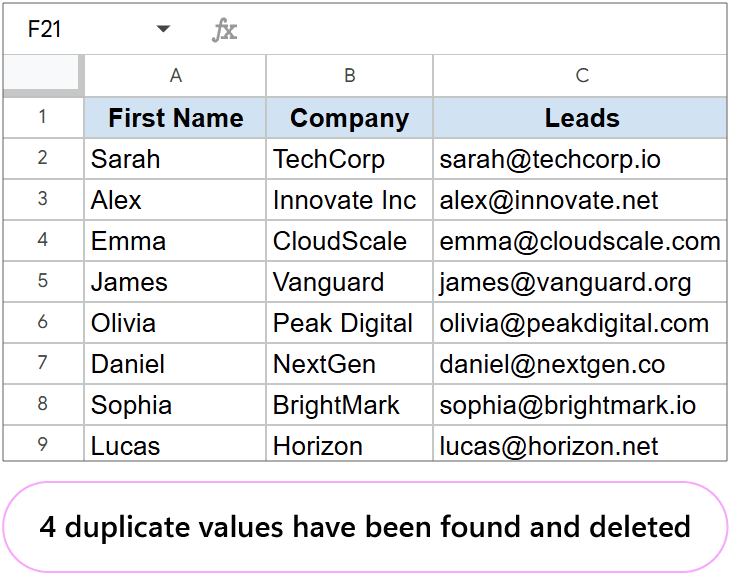
The Compare Columns tool identifies matching emails between two columns and automatically deletes unsubscribed contacts directly from your main list.
How it works:
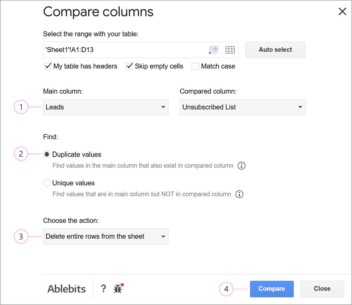
- Select your columns: Launch the add-on. Set the primary email list as the main column and the column with unsubscribed contacts as the compared column.
- Choose comparison mode: Select Duplicate values to target emails that exist in both columns.
- Select an action: Choose Delete entire rows from the sheet to remove unsubscribed emails together with related information.
- Run the tool: Click Compare.
Key benefits:
- Direct cleanup: Removes entire rows with unsubscribed contacts.
- No formulas needed: Replaces complex formula workarounds.
Case 3: Checking promo codes: case-sensitive comparison in Google Sheets
Scenario:
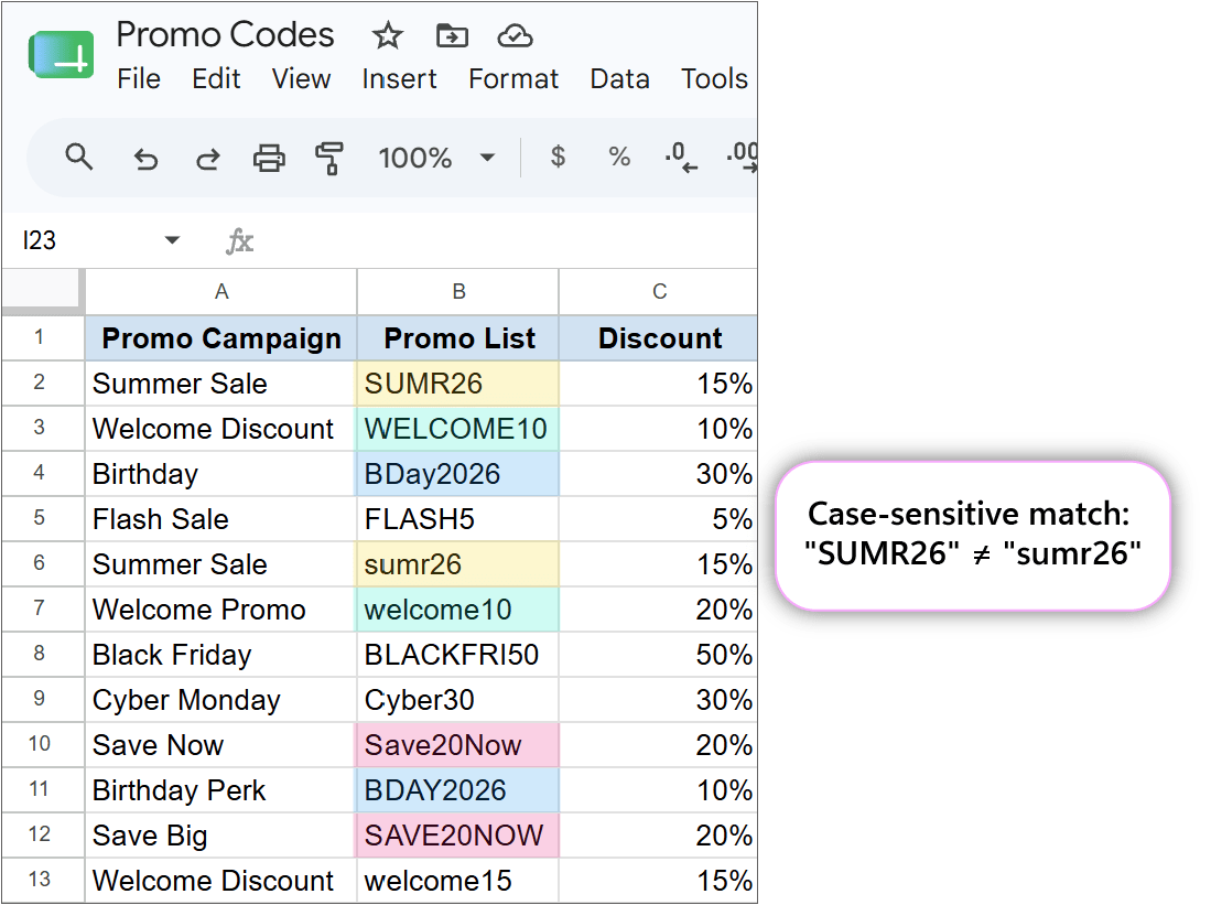
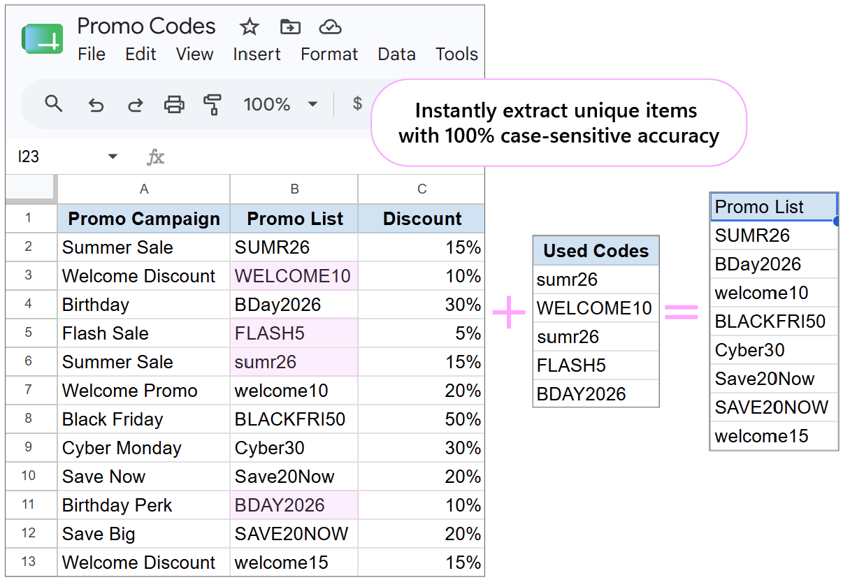
An e-commerce store manager receives an updated list of used promotional discount codes in one column and needs to extract all unused codes from their master list in another column. Since promo codes can be case-sensitive (e.g., “SUMR26” and “sumr26”), the lookup must accurately distinguish between uppercase and lowercase characters.
Problem:
- Case-insensitive default formulas: Standard Google Sheets functions like
=MATCH()or=COUNTIF()treat “SUMR26” and “sumr26” as identical values, leading to false matches. - Complex formula workarounds: To force a case-sensitive check using formulas, you have to build complex arrays combining
=EXACT()with=FILTER()or=ARRAYFORMULA(), which are hard to construct and maintain.
If you want to try this approach, you can read our guide on finding case-sensitive duplicates with formulas in Google Sheets (opens in a new tab).
Solution:
The Compare Columns tool includes a built-in Match case option, allowing you to run case-sensitive comparisons between two columns.
How it works:
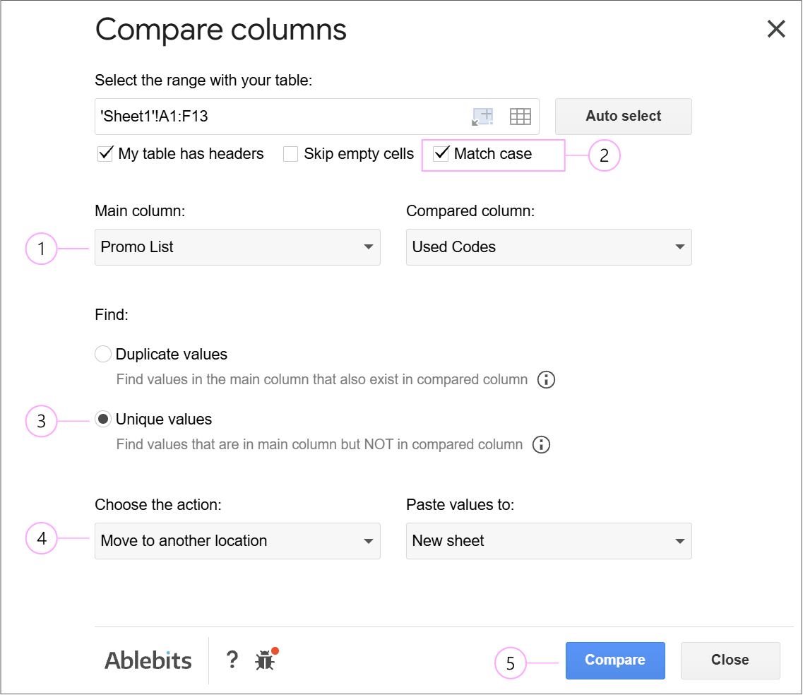
- Select your columns: Launch the add-on. Set the master promo code list as the main column and the list of used codes as the compared column.
- Enable case sensitivity: Check the Match case option to treat upper- and lowercase letters as distinct values.
- Choose comparison mode: Select Unique values to isolate codes that exist in your master list but are missing from the used codes list.
- Select an action: Choose Move to another location and select New sheet to generate a separate list of unused promo codes.
- Run the tool: Click Compare.
Key benefits:
- Exact matching: Easily differentiates between uppercase and lowercase letters without writing complex array formulas.
- Error prevention: Prevents valid promo codes from being incorrectly marked as used due to case-insensitive formula defaults.
- Export with ease: Automatically extracts unused codes to a new location.
Case 4: Extracting new products: compare two lists and copy unique values to new sheet
Scenario:
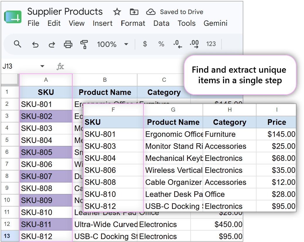
A retail manager receives an updated catalog from a supplier. They need to find new products that aren’t in their store yet and copy them to a separate spreadsheet to create new product cards, without altering or risking the master catalog.
Problem:
- Formula complexity: Pulling missing entries into a separate range using standard Google Sheets formulas requires constructing complex
=FILTER()or=ARRAYFORMULA(ISNA(MATCH(...)))statements. - Fragile links: Dynamic formulas remain linked to source cells. If supplier data is modified or cleared later, your extracted list of new items will break or return errors.
Solution:
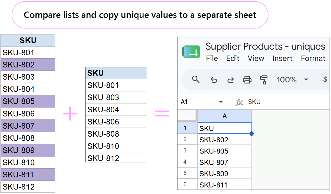
The Compare Columns tool compares both lists and uses the Copy to another location feature to safely export new items as static data to a new spreadsheet.
How it works:
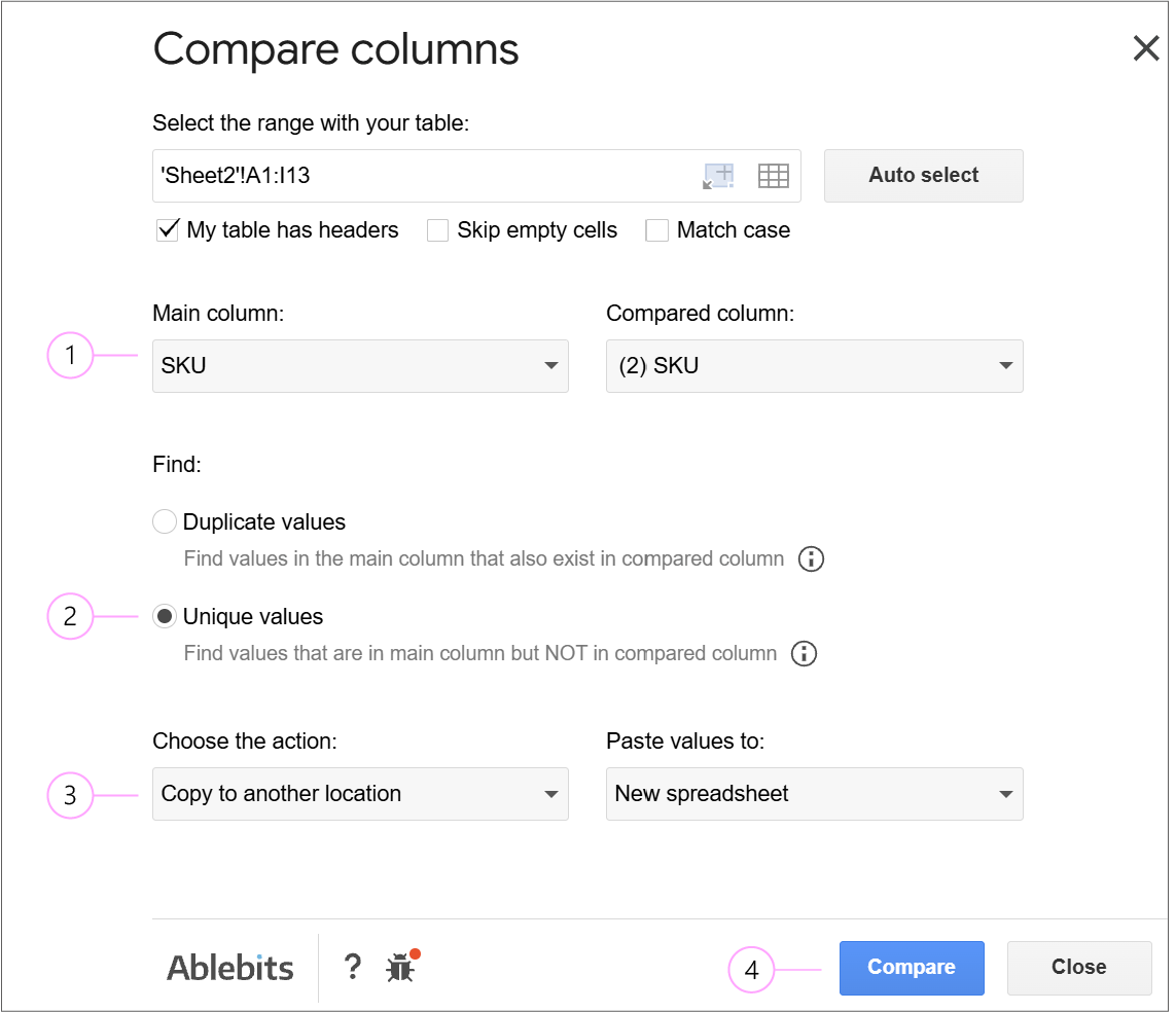
- Select your columns: Launch the add-on. Set your supplier’s list as the main column and the internal catalog list as the compared column.
- Choose comparison mode: Select Unique values to find products that exist only in the new supplier list.
- Select an action: Choose Copy to another location and select New spreadsheet.
- Run the tool: Click Compare.
Key benefits:
- Safe data extraction: Copies new records to a separate location without modifying, overwriting, or deleting original table data.
- Static results: Generates a clean, independent dataset that won’t break if source data changes.
- Zero coding: Eliminates the need to construct nested
=FILTER(ISNA())formulas.
Case 5: Tracking event attendance: compare two columns and add a status column
Scenario:
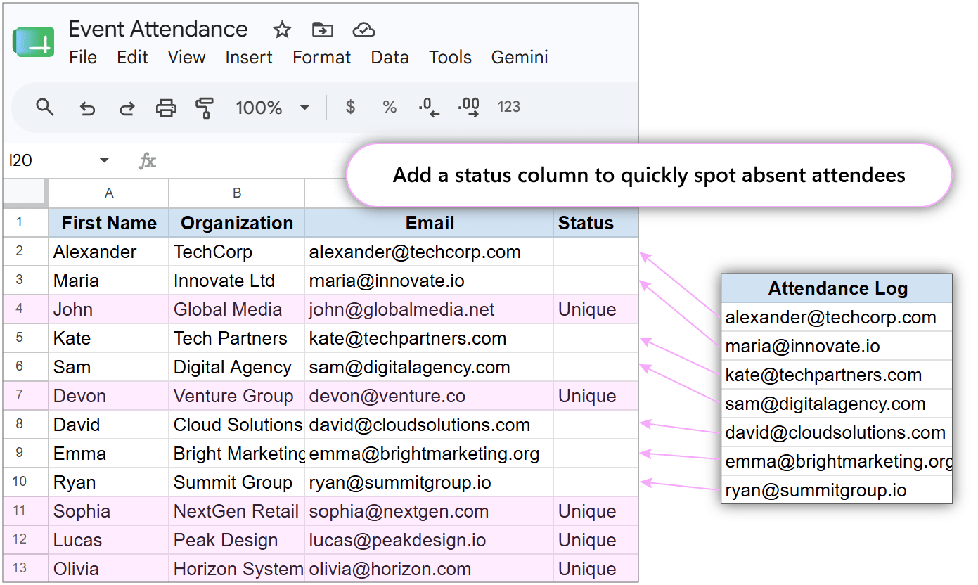
An event manager has a full list of registered participants in one column and an export list of actual attendees in another column. They need to review the entire main list to quickly spot who missed the event, keeping all original registrant records intact.
Problem:
- Formula hassle: Standard Google Sheets options like writing nested formulas (
=IF(ISNUMBER(MATCH(...)), "Attended", "")) require manual setup and dragging down thousands of rows. - Lack of clarity: You can color-code entries with conditional formatting, but color fills alone don’t give you explicit text tags if you want to scan attendance statuses by eye.
Solution:
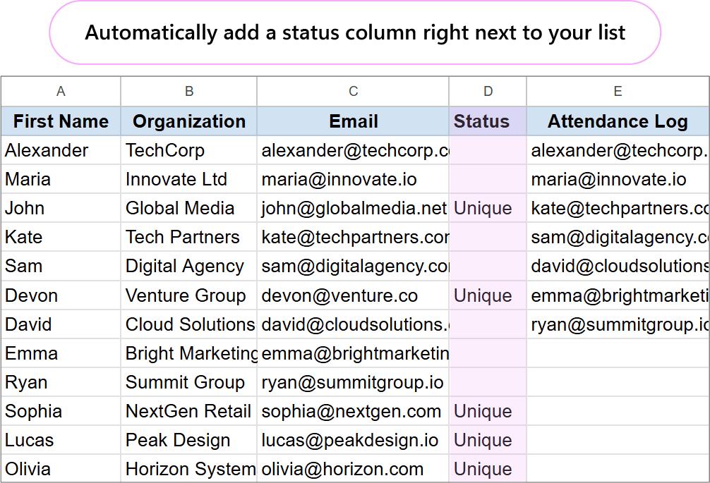
The Compare Columns tool automatically adds a Status column right next to your registrant list, adding status labels next to missing attendees.
How it works:
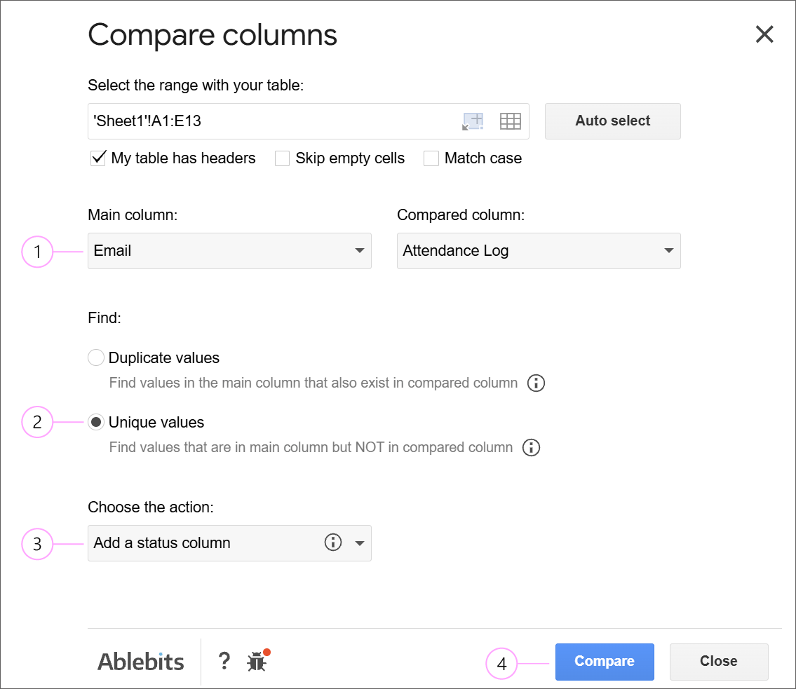
- Select your columns: Launch the add-on. Set the registered participants list as your main column and the actual attendees list as the compared column.
- Choose comparison mode: Select Unique values to target participants who registered but were missing from the attendee list.
- Select an action: Choose Add a status column to mark missing participants with a text label.
- Run the tool: Click Compare.
Key benefits:
- Clear overview: Instantly inserts text tags next to non-attending contacts, making absent participants easy to spot at a glance.
- Zero formulas: Replaces multi-step
=IF(MATCH())logic with simple, customizable status fields.
FAQ
How to compare two columns without using VLOOKUP or MATCH?
Use the Compare Columns tool (included with Compare Sheets or Power Tools) to find duplicates or unique values without writing formulas.
Is Ablebits Compare Columns safe?
Absolutely. We never see or analyze your spreadsheets.
Can I compare two columns across different sheets?
Yes, but you’ll need to use another tool: Compare Sheets for Duplicates (opens in a new tab). Compare Columns detects duplicates and unique values only in a single sheet.
How to compare two columns in Google Sheets and highlight differences?
Select your columns, set the comparison mode to Unique values, and choose Fill with color under actions.
Is there a case-sensitive column comparison in Google Sheets?
Yes, check the Match case option in the Compare Columns tool to differentiate between uppercase and lowercase values.
Ready to try it on your own spreadsheets?
Install Power Tools or Compare Sheets to access the Compare Columns tool and test all these features on your own data!
