
How to Merge and Combine Google Sheets: Use Cases

Learn how to merge two Google Sheets by key column and combine multiple tabs or files into one master sheet without VLOOKUP or complex formulas through real-world use cases.
Why Merge or Combine Google Sheets?
Main reasons to merge or combine sheets:
- Combining data: regional sales, financial statements, or department metrics into a master dashboard.
- Updating tables: prices, stock levels, or customer profiles with new information.
- Creating reports: complete datasets for pivot tables or executive analysis.
What’s the difference between merging and combining Google Sheets?
Let’s quickly look at how these two methods differ:
- Combining Sheets: Takes rows from multiple tabs or separate files and places them one below the other into a single master list based on matching column headers.
- Merging Sheets: Compares two tables using a shared key column (e.g., SKU or Email) and updates or transfers specific column values horizontally.
To handle both tasks, Ablebits offers two dedicated tools: Combine Sheets (opens in a new tab) and Merge Sheets (opens in a new tab).
Let’s look closer at how they operate:
| Combine Sheets | Merge Sheets | |
|---|---|---|
| How it works | Combines data from multiple sheets or files into a single master sheet. | Matches two tables by key column(s) to update matching rows or append new data. |
| Data alignment | Vertical: stacks data vertically based on matching column headers. | Horizontal: matches data horizontally using unique key column(s). |
| Best used for | Stack:
| Update:
|
| Formula alternative | =QUERY() | =VLOOKUP() or =XLOOKUP() |
- Use Combine Sheets when you want to stack rows vertically into a longer dataset.
- Use Merge Sheets when you want to match rows and update or add columns horizontally.
Case 1: Bulk update data in Google Sheets by key column
Scenario:
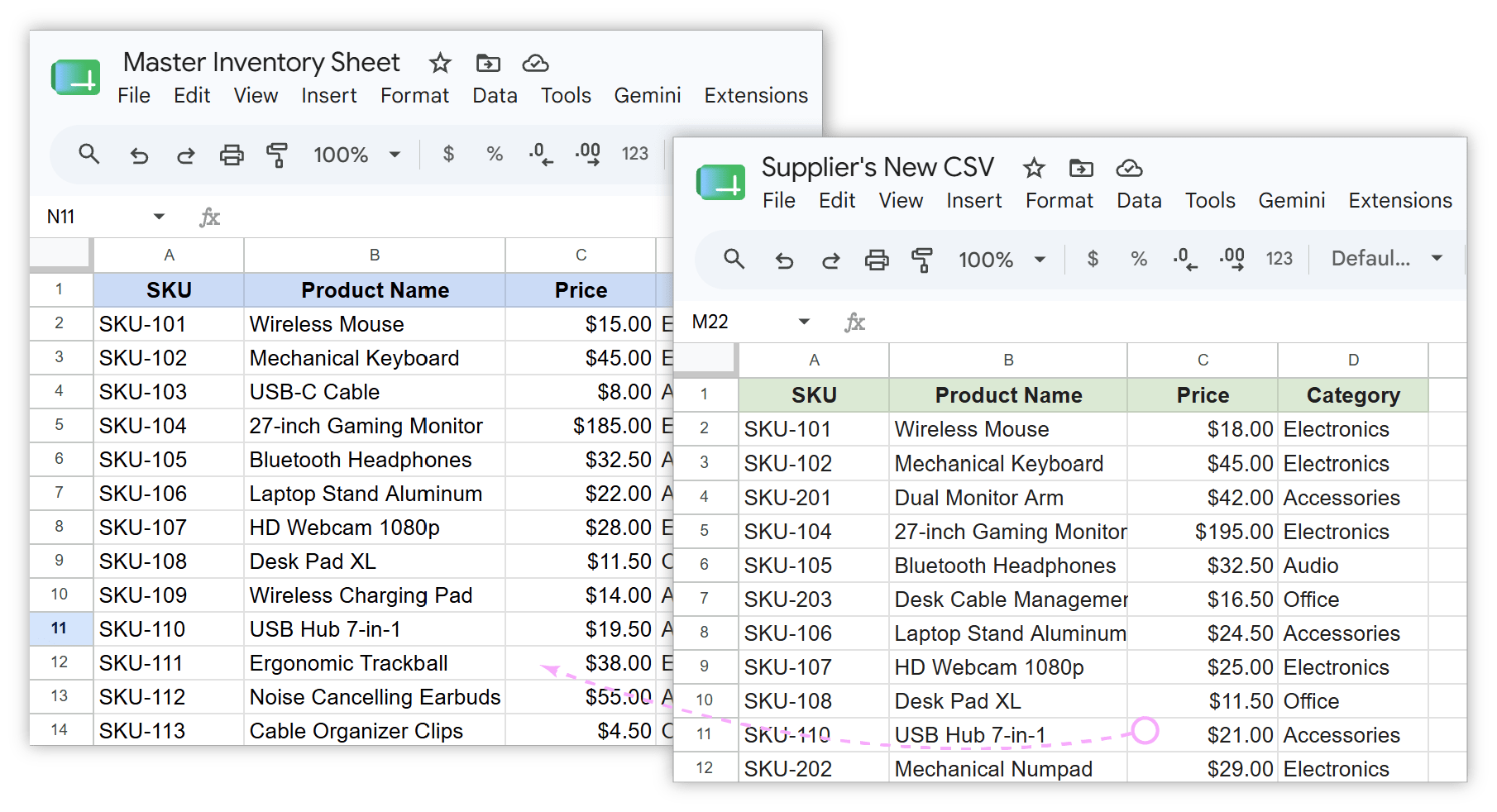
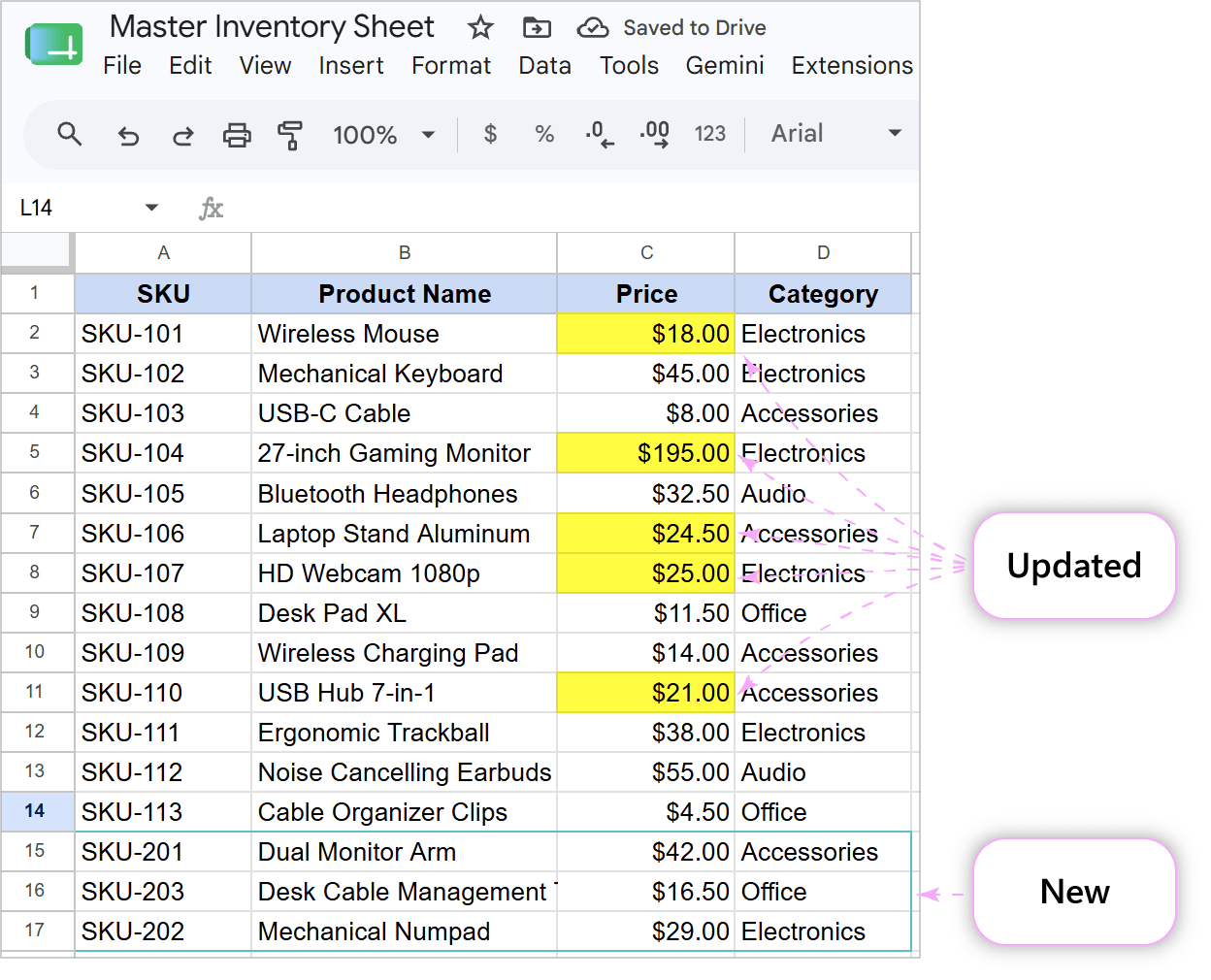
There is a master inventory sheet with over 5,000 items. The supplier sends a new price list with updated prices for 300 existing SKUs and 50 brand-new products. The goal is to update prices and stock levels for the matching SKUs and append the new items at the bottom.
Problem:
Updating an inventory sheet using standard Google Sheets formulas like =VLOOKUP() or =XLOOKUP() faces several serious problems:
- No direct overwriting: Formulas cannot update existing cell values in place. You have to insert temporary helper columns, pull the new prices, and manually copy-paste values over the old data.
- Complexity: Updating existing prices while simultaneously appending new product lines cannot be done in a single formula step without complex arrays.
- Fragile structure: If a team member deletes or reorders columns in the master sheet, formula range references break, causing errors across inventory logs.
Solution:
The Merge Sheets add-on updates existing records and appends new rows directly in your master inventory sheet.
How it works:
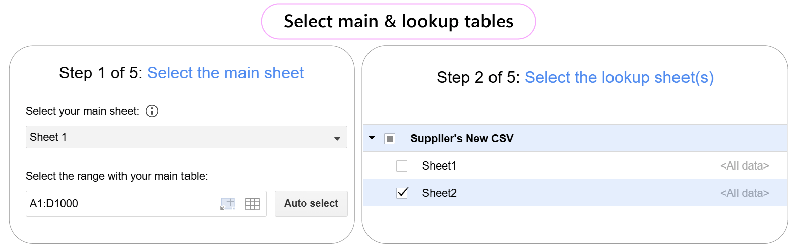
- Select your tables: Open your master sheet and launch Merge Sheets. Select your main table and the spreadsheet with the supplier’s updated data (your lookup table).
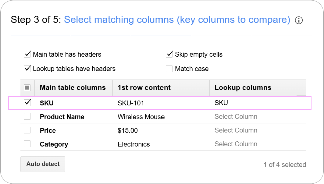
- Choose key columns: Select SKU as the matching key column to identify products across both sheets.
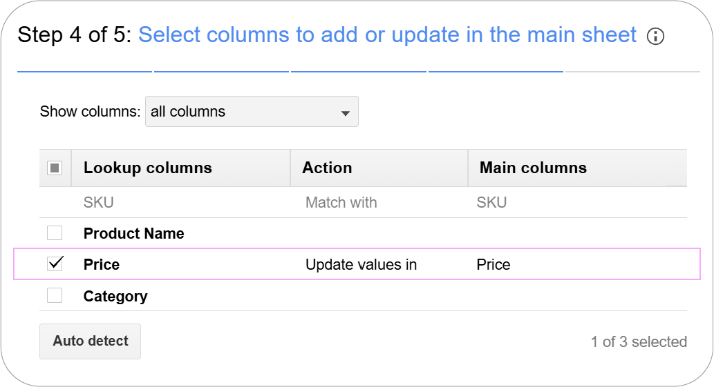
- Choose columns to update: Select the Price column to update existing values in place.
- Set rules:
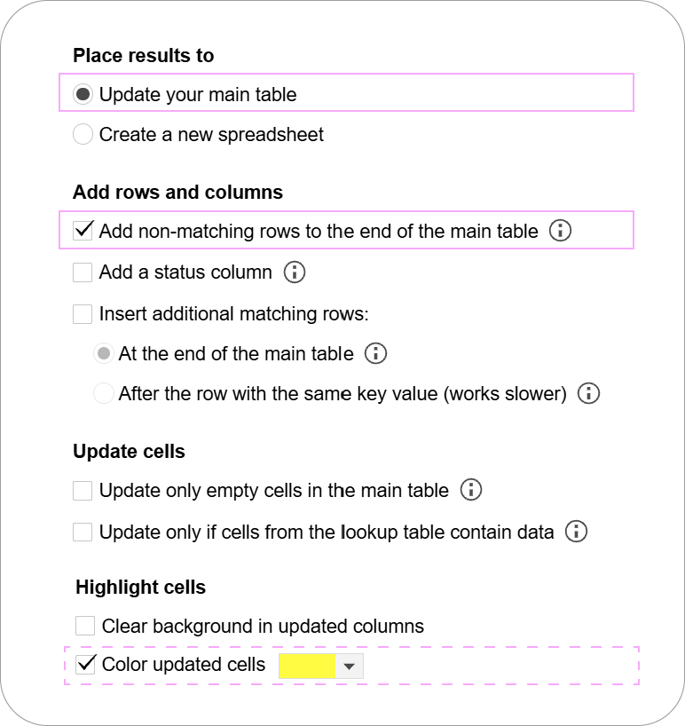
- Select the option Update your main table.
- Check Add non-matching rows to the end of the main table to automatically insert new product lines at the bottom.
- (Optional) Check the Color updated cells box to see all the changes.
- Run the extension: Click Merge.
Key benefits:
- Direct updates: Directly overwrites old prices in their original cells without temporary columns or manual copy-pasting.
- Two operations in one step: Updates existing SKUs and appends brand-new product lines simultaneously.
- Visual tracking: Includes an option to highlight updated cells in a custom color so you can quickly review changes.
Case 2: Combine multiple Google Sheets (or tabs) into one master sheet
Scenario:
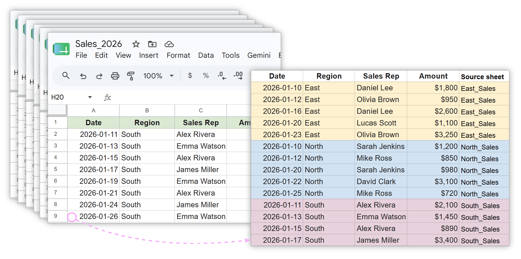
A sales director receives 12 individual monthly spreadsheets from 5 regional offices and needs to combine them into a single annual dataset.
Problem:
Combining multiple sales reports using native Google Sheets tools or manual work has its own hurdles:
- Manual errors: Stacking dozens of tabs by hand easily leads to missed rows, duplicated headers, and misplaced data.
- Complex chains: Linking multiple spreadsheets using nested arrays like
={IMPORTRANGE(...); IMPORTRANGE(...)}requires exact formula syntax and technical understanding.
A single misplaced bracket or comma breaks the entire master table. When I wrote a guide about the use of IMPORTRANGE (opens in a new tab), it took me a while to work out where and what had gone wrong, before I finally realised that I’d lost a bracket 🤦♀️.
- Loss of context: When stacking raw rows together, you lose track of which regional office or month a specific sale came from unless you manually add source tags to thousands of rows.
Solution:
The Combine Sheets add-on automatically pulls data from multiple tabs and separate Google Drive files, stacking them vertically into one continuous master table.
How it works:
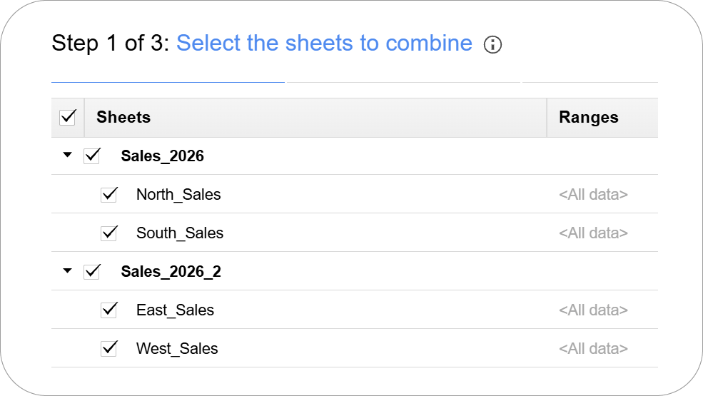
- Select your files and sheets: Launch Combine Sheets and select all 12 monthly sheets (or separate Google Drive files) at once.
- Select the columns to combine: You may check all or just several of them.
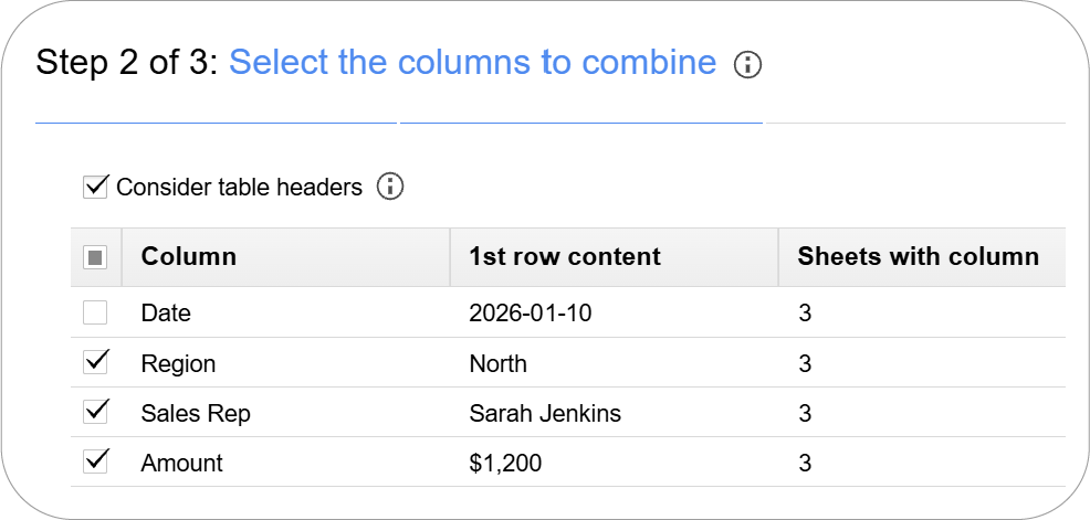
Do your regional sheets have columns in a different order? Check the Consider table headers option in that case. Combine Sheets will automatically match identical column headers across all files and stack data under the correct columns.
- Set the rules:
- Enable Add sheet names in a new column to the right to automatically tag each row with its source location.
- Choose how to sort the result.
- Select the place for your final dataset.
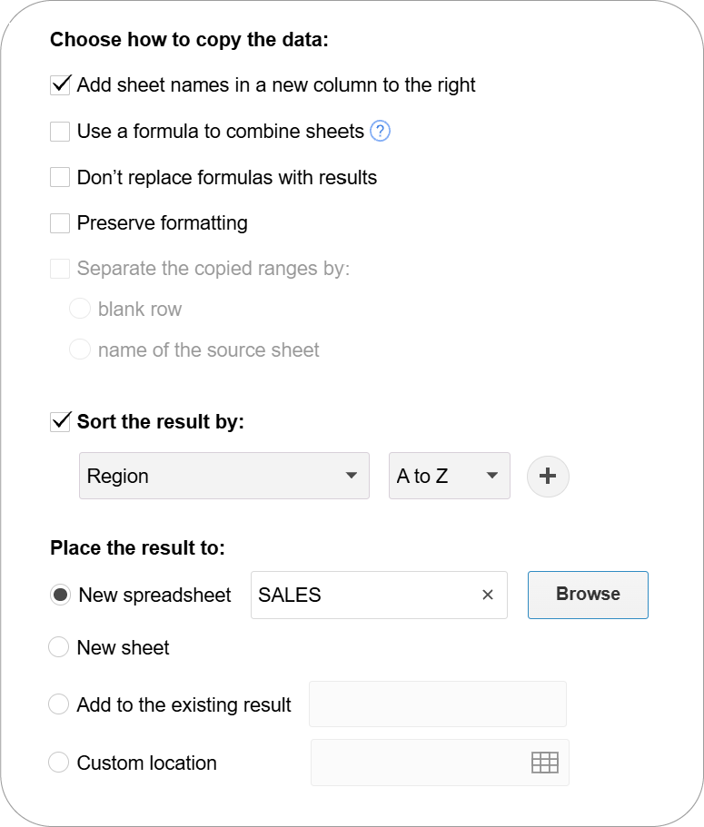
Need live auto-updates? By enabling the Use a formula to combine sheets option, your master table automatically pulls new rows and updates whenever regional reports change.
- Run the extension: Click Combine.
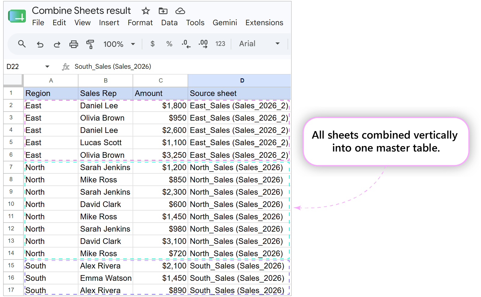
Key benefits:
- Easy combining: Stacks dozens of sheets or spreadsheets into one master dataset.
- Automatic header cleanup: Strips out repeating column headers automatically.
- Preserved context: Adds dedicated status columns showing the origin sheet or file name for every row.
- Auto-updates: Includes an option to refresh your combined data automatically whenever source sheets are updated.
Case 3: Merge two Google Sheets to enrich CRM data with new columns
Scenario:
There is a master CRM contact list in Google Sheets. After a recent webinar, the marketing team shares a new list of attendees with extra details like Job Title and Company Name. The goal is to enrich the existing contacts with these new data without ruining the master CRM structure or creating duplicate rows.
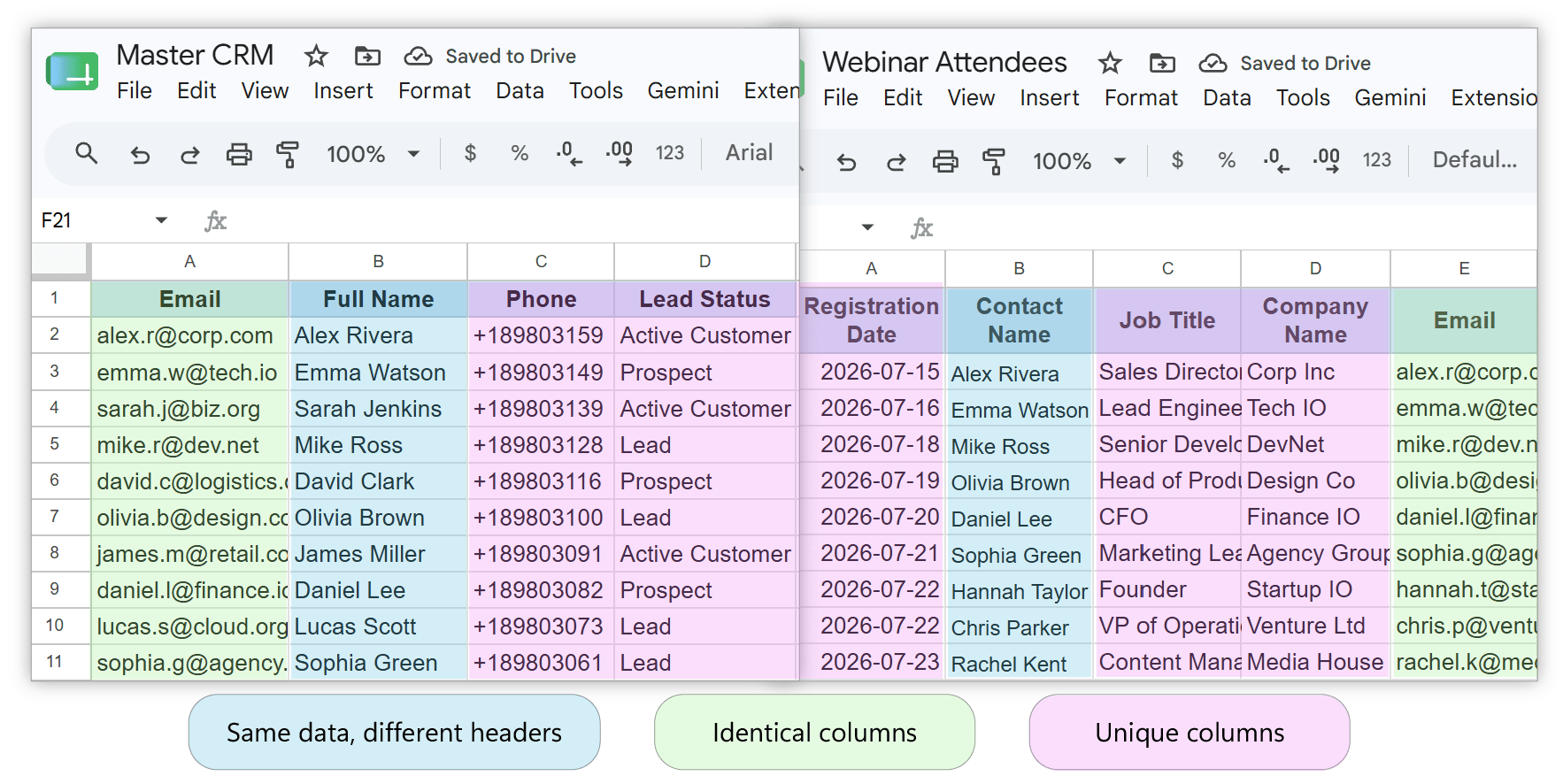
Moreover, the data in master CRM and table from the webinar is structured differently:
- In the master CRM table, there’s a column Full Name, while in the webinar sheet, the same column is named Contact Name.
- Columns appear in completely different order.
Problem:
Enriching an existing sheet with new data columns using standard Google Sheets tools creates several technical challenges:
- Formula limitations: Standard formulas like
=VLOOKUP()require identical key positioning or complex indexing. You have to manually insert empty new columns into the master sheet first and then construct lookup formulas for every new attribute. - Structural risk: Manually inserting columns and writing formulas across thousands of contacts risks misaligning rows or overwriting existing CRM fields like phone numbers or email addresses.
Solution:
The Merge Sheets add-on automatically matches contacts by a key column, creates new attribute columns in your master sheet, and populates them only for matching contacts.
How it works:
- Select your tables: Launch Merge Sheets and select your master CRM sheet (main table) and the webinar attendee file (lookup table).
- Choose key column: Select Email (or whatever matching columns you have) as the key column to link records across the tables.
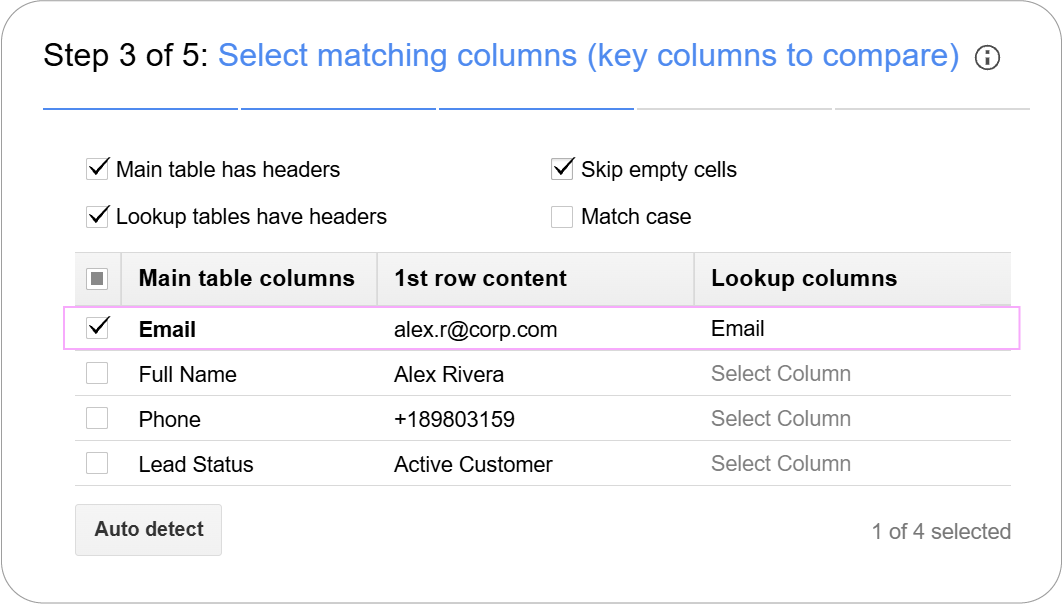
Use Auto detect to automatically match identical headers across tables.
- Choose columns to add or update: Select the new columns from the lookup table (e.g., Job Title, Company Name) to be added to your main table.
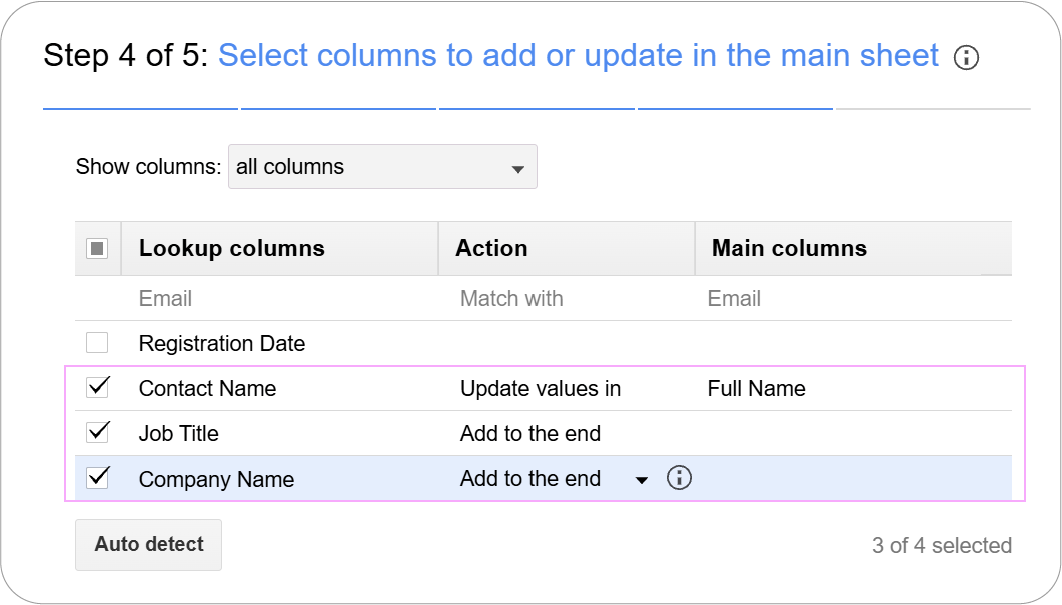
As you can see, I’ve manually paired columns with different headers but matching data (e.g., Contact Name with Full Name).
-
Set rules:
- Check Add non-existing columns to the end of the main table to automatically create and populate the new attribute columns.
- Check Update only empty cells in the main table to fill in missing names without touching existing CRM data.
-
Run the extension: Click Merge.
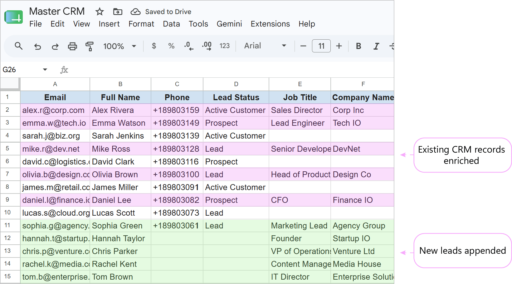
Key benefits:
- Flexible mapping: Merges data across tables with different header names or column sequences.
- Automatic column creation: Automatically creates and inserts new data columns into your master sheet.
- Safe data enrichment: Updates contact profiles while protecting existing CRM fields from being overwritten.
Case 4: How to automatically merge Google Sheets on a schedule
Scenario:
A logistics manager needs to reconcile daily warehouse shipments with online shop orders every morning at 10:00 AM. Each day, the warehouse system exports an updated list of shipped order IDs and tracking numbers to a Google Sheet. The goal is to automate this daily update so the master orders sheet refreshes on schedule without any manual work.
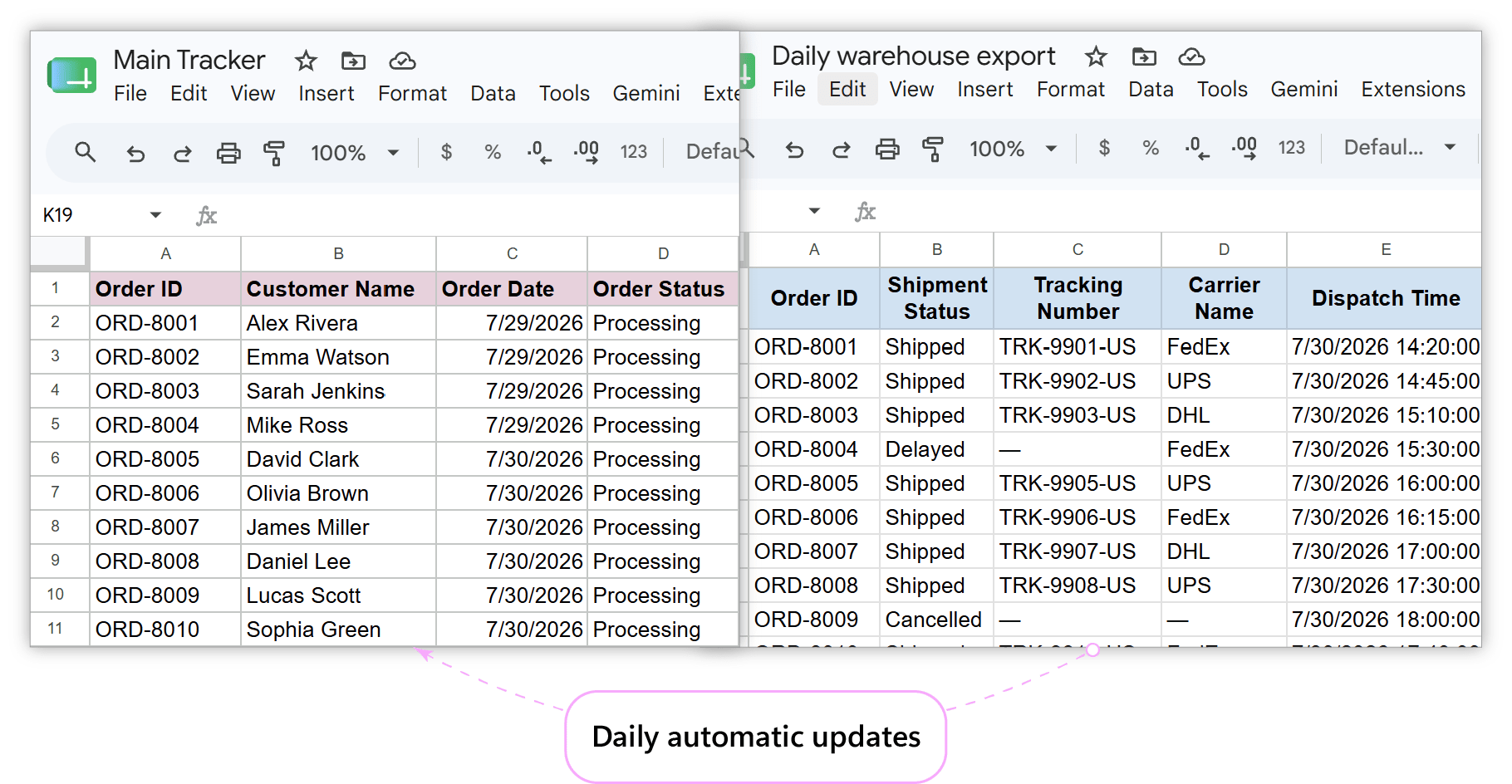
Problem:
Managing daily data reconciliation using standard Google Sheets features or basic tools has its own challenges:
- Manual work: Standard lookup formulas or basic add-ons require someone to physically open the spreadsheet, refresh range references, or manually run imports every day.
- Apps Script overhead: Custom Google Apps Script triggers can handle schedules, but they require ongoing code maintenance, API handling, and break easily when sheet structures change.
Solution:
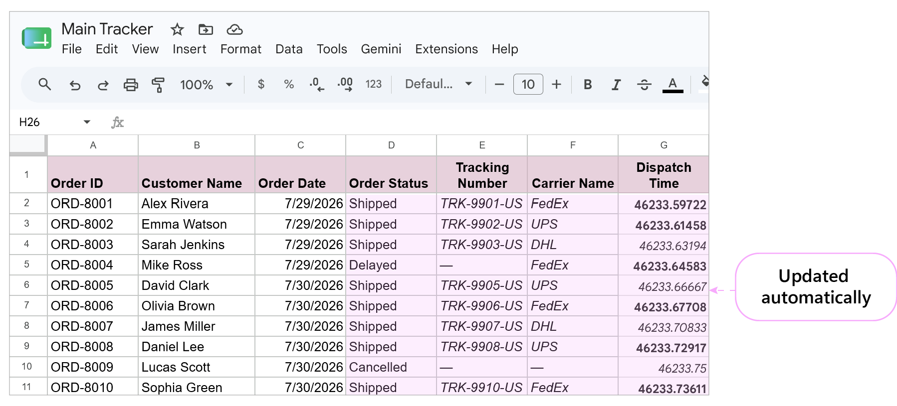
The Merge Sheets add-on allows you to schedule automated merge operations (e.g., daily at 10:00 AM). It runs in the background, updating order statuses and adding tracking numbers directly to your main table.
How it works:
- Set up the merge logic:
- Open Merge Sheets, select the main order table and the daily warehouse export as your lookup table.
- Select the matching key column (in our example, Order ID).
- Choose columns with attributes to update (Order Status, Tracking Number, Carrier Name).
- Set rules to update your main table and click Merge.
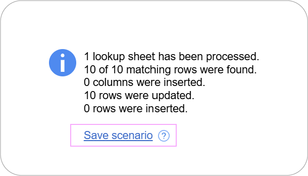
- Save as a scenario: After merging, save your configured options as a reusable scenario by clicking Save Scenario and entering a name for your rule (e.g., “Daily reconciliation”).
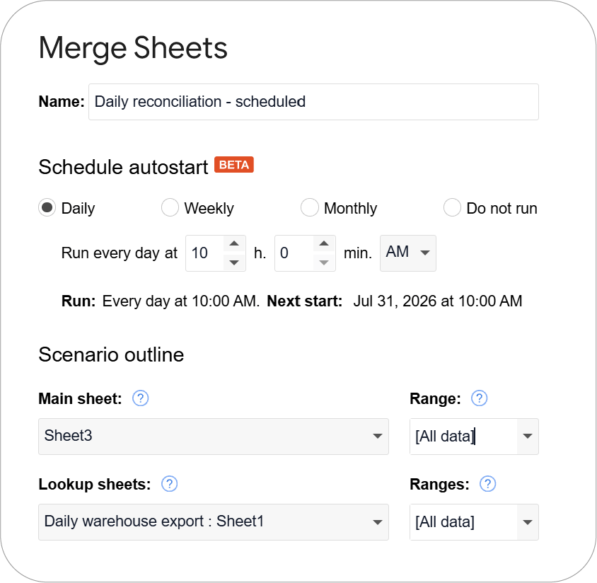
- Configure the schedule:
- Go to .
- Click your scenario and enable the automatic schedule trigger with the Set up recurring run button.
- Set the frequency to Daily, and specify the run time (10:00 AM).
- Save and activate: Click Create Schedule.
Key benefits:
- Automation: Runs automatically in the background on a timer without requiring anyone to open Google Sheets.
- No coding: Replaces complex Apps Script triggers with a simple, user-friendly schedule setup.
Why use Combine Sheets & Merge Sheets instead of formulas?
As these real-world use cases show, relying solely on standard Google Sheets formulas often leads to fragile setups, manual copy-pasting, and strict formatting limitations.
To help you decide which approach fits your workflow best, here is a direct comparison between standard Google Sheets formulas and the Ablebits Combine Sheets & Merge Sheets extensions:
| Feature / Criteria | Google Sheets Formulas (VLOOKUP, XLOOKUP, QUERY, IMPORTRANGE) | Ablebits Add-ons: Combine Sheets & Merge Sheets |
|---|---|---|
| Working with multiple spreadsheets | Tedious: Linking multiple spreadsheets requires long IMPORTRANGE(…); IMPORTRANGE(…) chains. | Seamless (Both tools): Select multiple separate Google Sheets files directly from Google Drive and combine or merge them into one sheet in a single click. |
| Handling missing data | Rigid: Formulas only return matching values; adding new non-matching rows requires separate complex logic or manual work. | Flexible:
|
| Overwriting existing data | Impossible: Formulas cannot directly overwrite existing cell values (you’ll need to create temporary helper columns). | Native support:
|
| Visual tracking | Manual: Highlighting changes or tracking status requires setting up complex Conditional Formatting rules and custom formulas. | Built-in:
|
| Auto-updating results | Complex setup: Creating live combined views requires nested QUERY + IMPORTRANGE arrays. In case of merging, daily or hourly updates require writing custom Google Apps Script code. | Built-in automation:
|
| Format preservation | Loses formatting: Standard formulas like QUERY or IMPORTRANGE pull only raw text/numbers, losing cell colors, borders, and number formats. | Preserves formatting:
|
| Ease of use | High curve: Requires memorizing and understanding exact syntax, nesting multiple functions, and handling formula syntax errors. | Convenient tool (Both tools): No technical expertise, code, or formula syntax required. |
FAQ
What methods can you use to merge or combine Google Sheets?
There are three main approaches depending on your technical skills and workflow needs:
- Formulas: Best for quick, simple joins on small datasets. However, the more scattered and complicated your data, the more nested formulas will become.
- Google Apps Script: Ideal for fully custom workflows, but requires coding expertise, API handling, and ongoing code maintenance.
- Add-ons: Best for fast, flexible, and automated combining & updates without coding. Extensions like Ablebits Merge Sheets & Combine Sheets handle simple data stacking as well as complex updates, mismatching columns, large datasets, and automatic scheduling.
How do I combine sheets in Google Sheets without formulas?
You can combine multiple sheets without writing formulas by using a no-code Google Sheets add-on like Ablebits Combine Sheets:
- Open your master spreadsheet and launch the add-on from the menu.
- Select the sheets to combine.
- Select the columns to combine.
- Set up extra options and click Combine.
The tool automatically consolidates all data, strips duplicate headers, and preserves formatting if needed.
How do I pull data from multiple tabs in Google Sheets?
To pull and stack data from multiple tabs into a single master sheet:
- Using Add-ons: Use Ablebits Combine Sheets to select all target tabs across your file, strip repetitive header rows, and insert a tracking column with the source tab name.
- Using Formulas: Use dynamic array brackets with the
QUERY()function. Note that native formulas require all tabs to have identical column structures.
How do I combine sheets with different column orders?
If your tables have matching data but different column layouts, use an add-on like Ablebits Combine Sheets:
- Launch Combine Sheets and select your target sheets or files.
- Check the Consider table headers option.
- Select the columns to combine and click Combine.
The add-on automatically aligns matching headers across all sheets and stacks identical columns together (even if they were in different positions).
How do I merge two Google Sheets based on a common column?
To join two tables using a unique key column (like SKU, Order ID, or Email):
- Open Ablebits Merge Sheets and select the sheet you want to update and the sheet with new data.
- Select the matching key column present in both tables (e.g., SKU).
- Choose which columns to update or pull into your main table.
- Set up extra options and click Merge to merge the tables in place without helper columns.
Can I combine Google Sheets from different files in Google Drive?
Yes. You can combine sheets stored across separate Google Drive files using two methods:
- Ablebits Combine Sheets: Select multiple separate Google Sheets files directly from your Google Drive folder and stack them into one sheet instantly.
- Native Formulas: Requires nesting multiple
IMPORTRANGE()functions inside array brackets.
Ready to combine and merge your Google Sheets without formulas?
